Data Structure - Big 0, Stack, Queue, Hashing, Sorting

Big O notation
Big O notation (with a capital letter O, not a zero), also called Landau's symbol, is a symbolism used in complexity theory, computer science, and mathematics to describe the asymptotic behavior of functions. Basically, it tells you how fast a function grows or declines.
Landau's symbol comes from the name of the German number theoretician Edmund Landau who invented the notation. The letter O is used because the rate of growth of a function is also called its order.
Sometimes, the number of basic operations depends on the input
▶ Best case: usually not relevant
▶ Average case: would require knowing distribution of inputs
▶ Worst case: easy to define, provides useful guarantee
-
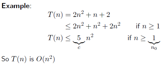
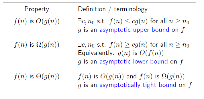
Big-O: Formal Definition
Big-O: expresses order of growth of the running time (basic number of operations) in the worst case
Definition: The function T(n) is O(f(n)) (read: “is order f(n)”) if there exist constants c > 0 and n0 ≥ 0 such that T(n) ≤ cf(n) for all n ≥ n0 (Functions represent running times, assumed nonnegative) We say that f is an asymptotic upper bound for T.
-
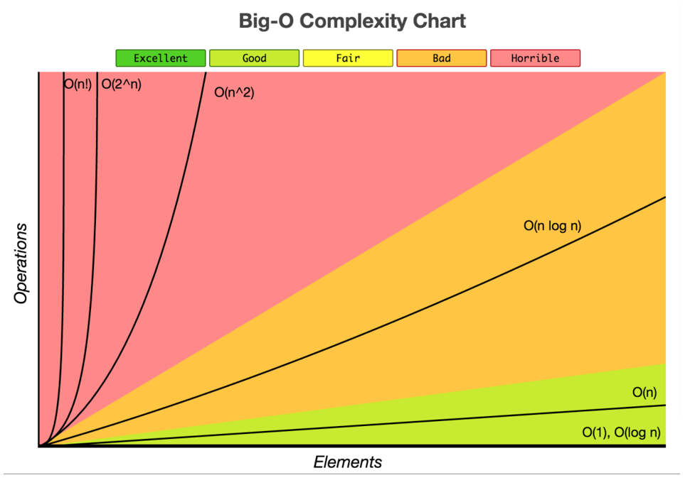
Big O Graph
In general we like to choose algorithms that work in O(1), O(log n) and O(n).We work with O(n log n) algorithms when we must.
We avoid algorithms with complexities beyond O(n log n). Typically problems that can only be solved by solutions that operate in high complexity have a monetary reward associated to them. You are rewarded if you solve it in a less complex manor. A problem worth $1 million.
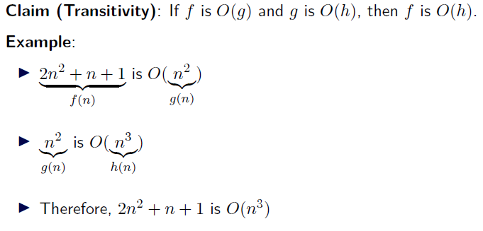
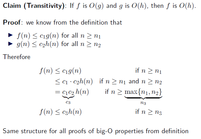
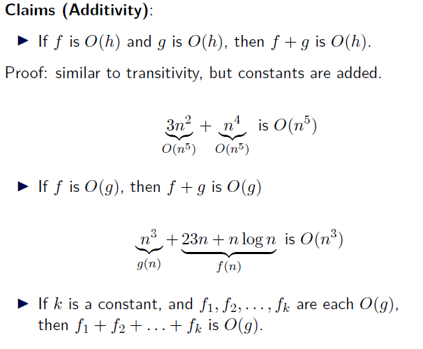
- Properties of Big-O: Transitivity
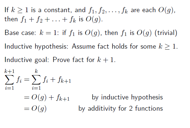
- Properties of Big-O: Additivity
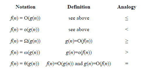
- Related Notation
-Asymptotics
Python Stack and Queue: Data structure organizes the storage in computers so that we can easily access and change data. Stacks and Queues are the earliest data structure defined in computer science. A simple Python list can act as a queue and stack as well. A queue follows FIFO rule (First In First Out) and used in programming for sorting. It is common for stacks and queues to be implemented with an array or linked list.
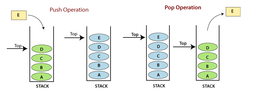
A Stack is a data structure that follows the LIFO(Last In First Out) principle. To implement a stack, we need two simple operations:
- push - which adds an element to the front of the stack.
- pop - which removes the first element in the the stack.
1 2 3 4 5 6 7 8 9 10 11 12 13 14 15 16 17 18 | class Stack: def __init__(self): self.stack = [] def push(self, x): self.stack.append(x) def pop(self): return self.stack.pop() if self.stack else -1 def size(self): return len(self.stack) def empty(self): return 1 if not self.stack else 0 def top(self): return self.stack[-1] if self.stack else -1 | cs |
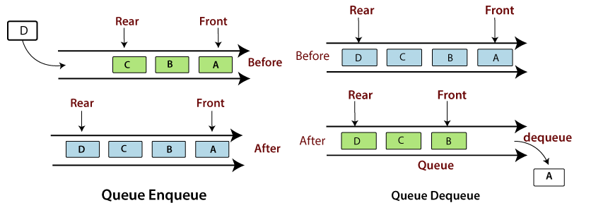
A Queue follows the First-in-First-Out (FIFO) principle. It is opened from both the ends hence we can easily add elements to the back and can remove elements from the front. To implement a queue, we need two simple operations:
- enqueue - It adds an element to the end of the queue.
- dequeue - It removes the element from the beginning of the queue.
1 2 3 4 5 6 7 8 9 10 11 12 13 14 15 16 17 18 19 20 21 22 23 24 25 | from collections import deque class Queue: def __init__(self): self.queue = deque() def push(self, x): self.queue.append(x) def pop(self): if self.queue: return self.queue.popleft() return -1 def size(self): return len(self.queue) def empty(self): return 1 if not self.queue else 0 def front(self): return self.queue[0] if self.queue else -1 def back(self): return self.queue[-1] if self.queue else -1 | cs |
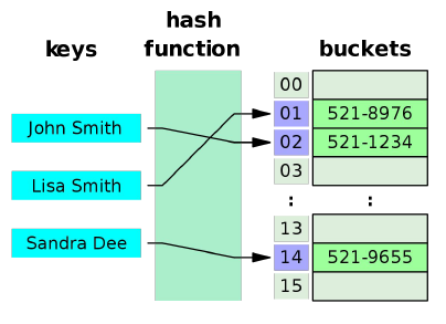
An array that stores pointers to records corresponding to a given Key.
An entry in hash table is Null if no value has been mapped to that existing index. In other words if no key value pair has not been put into the
table then the index mapps to a null value.
The same value may be mapped to different keys. But the same key may not be mapped to different values.
Why Do We Like Hashing?
Key Point: Hashing is the process of mapping a number to data. This number is
known as a key.
Hashing almost always leads to O(1) search times and O(n) in the VERY unlikely
worst case scenarios.
A good hash function should have the following properties:
- Efficiently computes key to their smaller number values. Often working in
O(1). - Should uniformly distribute the keys. This means that all keys produced by
the function should be equally likely to occur
1 2 3 4 5 6 7 8 9 10 11 12 13 14 15 16 17 18 19 20 21 22 | a = 100 b = 12.35 txt = 'Hello' print('Hash value of 100 is:', hash(a)) print('Hash value of 12.35 is:', hash(b)) print('Hash value of Hello is:', hash(txt)) # using dictionary students = {'cho': 17, 'lee': 15, 'park': 18} if 'cho' in students: print('cho is in students') else: print('cho is not in students') if 'son' in students: print('son is in students') else: print('son is not in students') >> 'cho' is in students >> 'son' is not in students | cs |
- Bubble Sort
A sorting algorithm that repeatedly steps through the list, compares adjacent elements and swaps them if they are in the wrong order. The process will repeatedly pass through the list until the list is sorted.
1 2 3 4 5 6 7 8 9 10 11 | for (int i =1; i < n; i++) { for (int j = 0; j < n-i; j++) { if (arr[j] > arr[j+1]) { swap(arr[j], arr[j+1]); } } } | cs |
Pros:
- imple to implement
- Efficient for (quite) small data sets
- Efficient for data sets that are partially sorted.
- Stable - does not change the relative order of elements with equal keys
- In-place - only requires no additional memory space, O(1)
Cons:
- Very bad for large data sets
- Not a practical sorting algorithm as its general less efficient than insertion sort on partially sorted set and no less complex.
- Computational Complexity:
- Best: O(n)
- Average: O(n^2)
- Worst Case:O(n^2 )
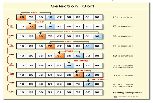
- Selection Sort
A sorting algorithm that is based on the idea of finding the minimum or maximum element in an unsorted array and then putting it in its correct position in another sorted array.
This option is inefficient on large lists, and generally performs worse than the similar insertion sort.
1 2 3 4 5 6 7 8 9 10 11 12 13 | for (int i =0; i < n-1; i++) { int min=i; for (int j = i+1; j < n; j++) { if (arr[j] < arr[min]) { min=j; } } swap(arr[i], arr[min]); } | cs |
Pros:
- Simple to implement
- Efficient for (quite) small data sets
- Stable - does not change the relative order of elements with equal keys
- In-place - only requires no additional memory space, O(1)
Cons:
- Very bad for large data sets
- Computational Complexity:
- Best: O(n^2)
- Average: O(n^2)
- Worst Case:O( n^2)
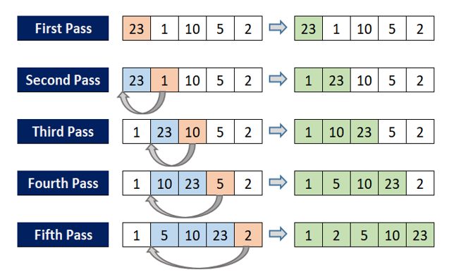
- Insertion Sort
A sorting algorithm where the sorted array is built comparing one item at a time. The array elements are compared with each other sequentially and then arranged simultaneously in a particular order.
1 2 3 4 5 6 7 8 9 10 11 12 | for (int i = 1; i < n-1; i++) { int key = arr[i]; int j = i; while (j > 0 && arr[j-1] > key) { arr[j] = arr[j-1]; j = j - 1; } arr[j] = key; } | cs |
Pros:
- Simple to implement, can be done with 3 lines of code
- Efficient for (quite) small data sets
- Efficient for data sets that are partially sorted. The time complexity is O(kn) when each element in the input is k places away from its sorted position.
- Stable - does not change the relative order of elements with equal keys
- In-place - requires no additional memory space, O(1)
- Online - can sort a list as it receives it
Cons:
- Very bad for large data sets
- Computational Complexity:
- Best: O(n)
- Average: O(n^2)
- Worst Case: O(n^2)
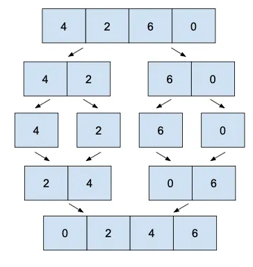
- Merge Sort
The algorithm repeatedly breaks down a list into several sublists until each sublist consists of a single element and merging those sublists in a manner that results into a sorted list.
One of the most efficient sorting algorithms.
Can be developed recusively
1 2 3 4 5 6 7 8 9 10 | ALGORITHM MERGESORT(A, low, high) If (low < high) then Mid= (low + high)/2 MERGESORT(A, low, mid) MERGESORT(A,mid + 1, high) MERGE(A,low, mid, high) End If End MERGESORT Recursion | cs |
Pros:
- Time-efficient
- Highly parallelizable
- Stable - does not change the relative order of elements with equal keys
Cons:
- Not online, you cannot sort array while it is received
- More complicated to code
- Not in-place, it requires additional memory space.
- Marginally slower than quicksort in practice
Computational Complexity:
- Best: O(n log(n))
- Average: O(n log(n))
- Worst Case: O(n log(n))
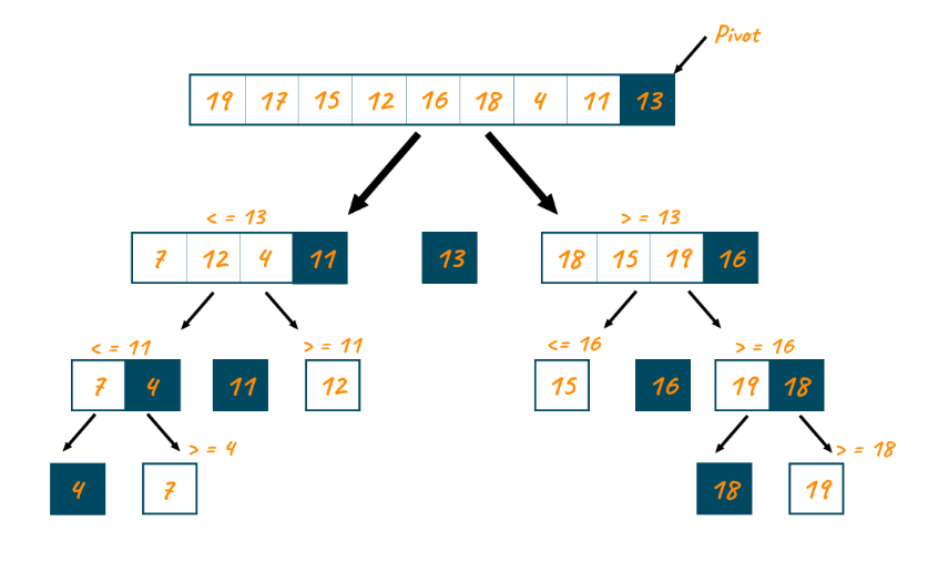
- Quick Sort
A highly efficient sorting algorithm that is a divide-and-conquer approach based on the idea of choosing one element as a pivot element (See subsequent slides for pivot selection) and partitioning the array around it such that:
Left side of pivot contains all the elements that are less than the pivot element
Right side contains all elements greater than the pivot
Also known as Partition-Exchange Sort
The most practical sorting algorithm as it reduces space complexity and removes the use of the auxiliary array that is used in merge sort.
1 2 3 4 5 6 7 8 9 10 11 12 13 14 15 16 17 18 19 20 21 22 23 24 25 | partition(A,l,h) { pivot=A[l]; i=l; j=h; while(i<j) { while(A[i]<=pivot) i++ while(A[j]>pivot) j--; If(i<j) swap(A[i],A[j]); } if(i>j) swap(A[l],A[j]); return j; } quicksort(A,l,h) { if(l<h) { p=partition(l,h) quicksort(A,l,p-1); quicksort(A,p+1,h); } } | cs |
Pros:
- Time-efficient
- Highly parallelizable
- In-place - requires no additional memory space, O(1). Thus it can be about two or three times faster than its main competitors, merge sort and heapsort
- Stable - does not change the relative order of elements with equal keys
Cons:
- Not online, you cannot sort array while it is received
- More complicated to code
Computational Complexity:
- Best: O(n log(n))
- Average: O(n log(n))
- Worst Case: O(n^2)
- Heap Sort
A sorting algorithm that builds a Heap data structure from the given array and then utilizing the Heap to sort the array.
Heap is a special binary search tree, that satisfies the following special heap properties:
1)Shape Property: Heap data structure is always a Complete Binary Tree, which means all levels of the tree are fully filled.
2)Heap Property: All nodes are either greater than or equal to or less than or equal to each of its children.
○ Max-Heap when the parent nodes are greater than their child nodes,
○ Min-Heap when the parent nodes are smaller than their child nodes
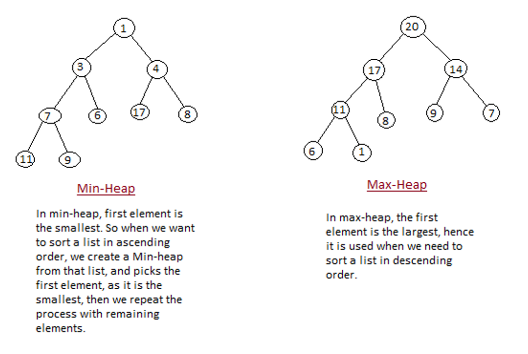
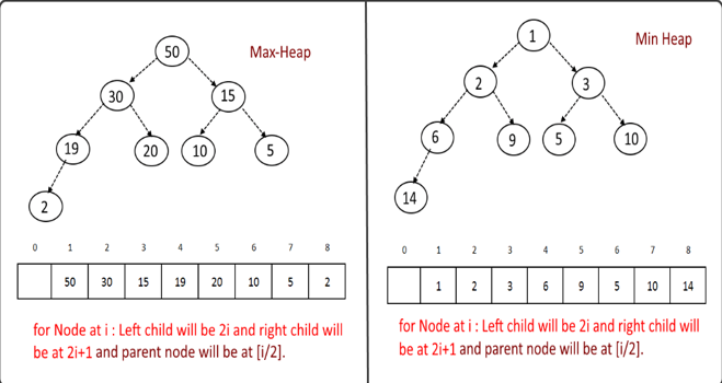
Heap Property: All nodes are either greater than or equal to or less than or equal to each of its children. If the parent nodes are greater than their child nodes, heap is called a Max-Heap, and if the parent nodes are smaller than their child nodes, heap is called Min-Heap
1 2 3 4 5 6 7 8 9 10 11 12 13 14 15 16 17 18 19 20 | MaxHeapify(A, i) l <- left(i) r <- right(i) if l <= heap-size[A] and A[l] > A[i] then largest <- l else largest <- i if r <= heap-size[A] and A[r] > A[largest] then largest <- r if largest != i then exchange A[i] <-> A[largest] MaxHeapify(A, largest) HeapSort(A) Build-Max-Heap(A) for i <- length[A] downto 2 do exchange A[1] <-> A[i] heap-size[A] <- heap-size[A] – 1 MaxHeapify(A, 1) | cs |
Pros:
- Time-efficient
- In-place - only requires no additional memory space, O(1). A heap is just a bunch of pointers.
Cons:
- Not online, you cannot sort array while it is received
- More complicated to code
- Marginally slower than quicksort in practice
Computational Complexity:
- Best: O(n log(n))
- Average: O(n log(n))
- Worst Case: O(n log(n))
Priority Queue:
- Popular & important application of heaps.
- Max and min priority queues.
- Maintains a dynamic set S of elements.
- Each set element has a key – an associated value.
- Goal is to support insertion and extraction efficiently.
- Applications:
»Ready list of processes in operating systems by their priorities – the list is highly dynamic
»In event-driven simulators to maintain the list of events to be simulated in order of their time of occurrence.
 IlMinCho


